3.2 The SceneGrid Class
3.2.1 Definition
This class represents the 2-dimensional discretisation of a surface. It can be used for instance to describe a focal plane.
The surface coordinates are called world coordinates and the pixelised ones the pixel coordinates. The adopted convention is that the coordinates of the bottom-left pixel center is (0, 0).
Currently, the world-to-pixel transform is specified through a FITS header.
>>> header = create_fitsheader((256, 256), cdelt=250, cunit='um', crval=(0, 0),
                               ctype=['X---CAR', 'Y---CAR'])
>>> plane = SceneGrid.fromfits(header)
>>> print plane.topixel((0, 0))
[ 127.5  127.5]
>>> print plane.toworld((0, 0))
[-31875. -31875.]
3.2.2. Use in conjonction with the Layout class
Let’s consider an array of detectors placed on the detector focal plane. The Layout will collect information on the individual detectors, but it bears no information on how the focal plane is discretised. It’s precisely the purpose of the SceneGrid class. The detector Layout instance can be created so that the detector positions are expressed in the world coordinates of the SceneGrid instance associated with the focal plane. By doing so, it will be easy to compute the coordinates of the detector centers or corners in the detector plane pixel coordinates.
>>> layout = LayoutGridSquares((8, 8), Quantity(200, 'um'))
>>> header = create_fitsheader((64, 64), cdelt=25, cunit='um', crval=(0, 0),
                               ctype=['X---CAR', 'Y---CAR'])
>>> plane = SceneGrid.fromfits(header)
>>> print(plane.topixel(layout.all.center[7,0]))
[ 3.5  3.5 ]
>>> print(plane.topixel(layout.all.vertex[7,0,2]))
[-0.5 -0.5]
3.2.3. Polygon intersections
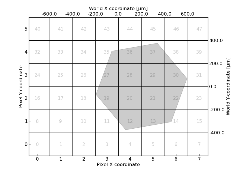
The SceneGrid class facilitates the computation of the intersections between polygons (usually detector squares) and the pixels of a discretised surface. Let’s assume that we are dealing with a hexagon-shaped detector. We are interested in determining which pixels it intersects and quantify the intersected fraction for each of them. This information is computed through a projection Operator, which has a detector plane array as input \( x \) and the integration inside the detector polygon as output \( y \). Both of them are related through:
\[
y = \sum_j P_{j}\,x_j
\]
where \( P_j \) denotes the fraction of pixel \( j \) intersected by the detector.
>>> from pysimulators.geometry import create_regular_polygon
>>> nx, ny = 8, 6
>>> header = create_fitsheader((nx, ny), cdelt=200, cunit='um', crval=(0, 0),
...                            ctype=['X---CAR', 'Y---CAR'])
>>> plane = SceneGrid.fromfits(header)
>>> polygon = create_regular_polygon(6, 400, angle=10, center=(200, 0))
>>> fig = figure()
>>> ax = fig.add_subplot(111)
>>> ax.add_patch(Polygon(plane.topixel(polygon), closed=True, alpha=0.2,
...                      color='k'))
>>> indices = np.arange(nx * ny)
>>> for (x, y), s in zip(plane.toNd(indices), indices):
>>>     text(x, y, s, horizontalalignment='center',
...          verticalalignment='center', alpha=0.2)
>>> ax.set_xlabel('Pixel X-coordinate')
>>> ax.set_ylabel('Pixel Y-coordinate')
>>> for i in range(nx-1):
...     ax.axvline(i+0.5, color='k')
>>> for i in range(ny-1):
...     ax.axhline(i+0.5, color='k')
>>> ax2 = ax.twiny()
>>> ax2.set_xticks(np.arange(nx-1) + 0.5)
>>> ax2.set_xticklabels(np.linspace(-600, 600, nx-1))
>>> ax2.set_xlabel(u'World X-coordinate [µm]')
>>> ax3 = ax.twinx()
>>> ax3.set_yticks(np.arange(ny-1) + 0.5)
>>> ax3.set_yticklabels(np.linspace(-400, 400, ny-1))
>>> ax3.set_ylabel(u'World Y-coordinate [µm]')
>>> for a in (ax, ax2, ax3):
...     a.set_xlim(-0.5, nx - 0.5)
...     a.set_ylim(-0.5, ny - 0.5)
...     a.set_aspect('equal')
The sparse matrix \( P \) can be accessed through the matrix attribute. It contains information on the intersected pixels: matrix.data.index is the 1-dimensional pixel index and matrix.data.value is the fraction of the pixel intersected by the polygon, ranging from 0 if there is no overlap to 1 if the polygon encompasses the surface pixel.
>>> proj = plane.get_integration_operator(plane.topixel(polygon))
>>> proj.matrix.ncolmax  # number of pixels intersected by the hexagon
16
>>> data = proj.matrix.data.squeeze()
>>> for k, (x, y), v in zip(data.index, plane.toNd(data.index), data.value):
...     print('{} => ({}, {}) : {}'.format(k, x, y, v))
11 => (3, 1) : 0.106081987181
12 => (4, 1) : 0.778645861985
13 => (5, 1) : 0.670606992789
14 => (6, 1) : 0.210664784161
19 => (3, 2) : 0.768927943509
20 => (4, 2) : 1.0
21 => (5, 2) : 1.0
22 => (6, 2) : 0.661224853081
27 => (3, 3) : 0.661224853081
28 => (4, 3) : 1.0
29 => (5, 3) : 1.0
30 => (6, 3) : 0.768927943509
35 => (3, 4) : 0.210664784161
36 => (4, 4) : 0.670606992789
37 => (5, 4) : 0.778645861985
38 => (6, 4) : 0.106081987181
We can check that the sum of the intersected fractions
>>> sum(proj.matrix.data.value)
10.392303
is equal to the area \( A \) of the hexagon, in units of pixels. Recalling that the hexagon center-to-vertex distance is 400 µm and that the pixel size is 200 µm:
\[
A = \frac{3\sqrt{3}}{2}\times \left(\frac{400}{200}\right)^2\approx 10.39230
\]
The reason why an Operator is obtained from the SceneGrid instance (instead of the sparse matrix), is that integration inside a detector is simply performed by calling the operator. In the case of a flat field (but any values for the surface could be used) it would be written as:
>>> print(proj(np.ones((ny, nx))))
10.3923047632